Scrape the data

Gosh webscraping is very moreish when you get into it. This is how I got hold of all the lyrics on (almost) every song on all 100 albums, sort of quickly.¹

The Now! series has a website with a page giving track listings for every album, and the URLs follow a fairly regular pattern, the only slight inconvenience being the different format of the URL for numbers 1 and 97-100. From there it’s full steam ahead for extracting the info with rvest and coercing it into the shape I want in a dplyr pipeline.

library(tidyverse)
library(rvest) 
library(glue)

get_tracks <- function(n) { 
  
  if(n < 97) {
    if(n ==1){
      url <- glue("http://www.nowmusic.com/album/now-thats-what-i-call-music/")
    } else {
      url <- glue("http://www.nowmusic.com/album/now-thats-what-i-call-music-",n,"/")
    }
  } else {
    url <- glue("http://www.nowmusic.com/album/now-",n,"/") 
  }
  
  songdata <- read_html(url) %>% 
    html_nodes("ul li p")
  
  alblen <- length(songdata) / 3
  
  tracklist <- bind_rows(lapply(html_text(songdata), 
                                function(x) data.frame(x, stringsAsFactors = FALSE))) %>% 
    mutate(type = rep(1:3, alblen), id = rep(1:alblen, each = 3)) %>% 
    group_by(type, id) %>% 
    mutate(id2 = row_number()) %>% 
    spread(type, x) %>% 
    mutate(track = id, song = `2`, artist = `3`) %>% 
    select(track, song, artist)
}

# Use this to get track listings for all 100 tracks

nows <- c(1:100)
nowalbums <- lapply(nows, get_tracks)

Now for the lyrics, which come from the genius.com website. It has an API for extracting them, but fortunately there is an R package for quick n easy scraping so I can get away with still not really understanding what APIs are or how to use them. The geniusR package is based on generating the lyrics URL from the artist and song title, which I conveniently have thanks to the previous scraping exercise. It mostly works, but not always. Some quirks are relatively easy to deal with - removing ‘featured’ artists or punctuation from song titles improves things considerably. Accented letters can be changed to non-accented ones, although it’s harder to make a rule to deal with punctuation within a name, like P!nk. The code here generally fails to match about five songs on each album, so in the absence of spending any further time on data processing, the final dataset will be missing a few things, including sadly all of P!nk’s ouvre.

library(geniusr)

# Function that extracts lyrics for a given track number on a given NOW album number

getlyric <- function(tn, an) {
  artist <- gsub(" feat\\..*", "", nowalbums[an][[1]][tn,4])
  artist <- gsub(" x ", " and ", artist)
  artist <- gsub(" FT.*", "", artist)
  artist <- gsub("[^[:alnum:][:space:]&-]", "", artist)
  artist <- iconv(artist, from = "UTF-8", to = "ASCII//TRANSLIT")
  song <- gsub("[^[:alnum:][:space:]&]", "", nowalbums[an][[1]][tn,3])
  genius_lyrics(artist, song) %>% 
    spread(line, lyric) %>% unite("lyrics", -1, sep = " ")
}

# Function that fetches all lyrics for a given album

lyrictbl <- function(an) {
  nums <- c(1:nrow(nowalbums[an][[1]]))
  tbllist <- lapply(nums, function(x) try(getlyric(x, an)))
  do.call(rbind, tbllist) %>% 
    mutate(track = row_number()) %>% 
    mutate(lyrics = replace(lyrics, lyrics == "Error in read_xml.response(x$response, ..., as_html = as_html) : \n  Not Found (HTTP 404).\n", NA)) 
}

# Function to fetch track listing and lyrics for given album and bind together

lyrictable <- function(n) {
  albumlyrics <- lyrictbl(n)
  full_join(nowalbums[n][[1]], albumlyrics, by = "track") %>% 
    mutate(alb = n) %>% 
    select(track, song, artist, lyrics, alb)
}

# Bind everything in one monster table

nums <- c(1:100)
alllyric <- bind_rows(lapply(nums, lyrictable))

Finally I want to merge in information about release date, because I think date is a more meaningful scale for measuring these trends than album numbers. I scraped this from the relevant Wikipedia page about the albums.

library(lubridate)

# Import release date from wikipedia

url <- "https://en.wikipedia.org/wiki/Now_That%27s_What_I_Call_Music!_discography#United_Kingdom_and_Ireland"

dates <- read_html(url) %>% 
  html_nodes("tr td") %>% 
  html_text()

lines <- seq(4,499,5)

datelist <- bind_rows(lapply(lines, function (x) as_tibble(dates[x]))) %>% 
  mutate(value = gsub("\n", "", value)) %>% 
  mutate(date = dmy(value)) %>% 
  mutate(id = row_number(), alb = paste0("now",id)) %>% 
  mutate(alb = gsub("now", "", alb)) %>% 
  mutate(alb = as.integer(alb)) %>% 
  select(alb, date)

# Merge dates with info and create decade variable

lyricdata <- alllyric %>% 
  select(track, song, artist, lyrics, alb) %>%
  full_join(datelist) %>% 
  mutate(decade = floor_date(date, years(10)))%>% 
  mutate(decade = factor(decade)) %>% 
  mutate(decade = recode(decade, "1980-01-01" = "1980s",
                                  "1990-01-01" = "1990s",
                                  "2000-01-01" = "2000s",
                                  "2010-01-01" = "2010s"))

A lyrical evolution

An easy one first; what was the most popular word in each decade? I’m measuring popularity here as a proportion – the number of times a word appeared relative to the total words (after removing boring words like ‘the’).

library(tidytext)

lyricsdata %>% 
  group_by(decade) %>% 
  unnest_tokens(word, lyrics) %>% 
  anti_join(stop_words) %>%
  count(word) %>% 
  mutate(prop = n / sum(n)) %>% 
  arrange(decade, desc(prop)) %>% 
  top_n(20) %>% 
  mutate(word = as.factor(word)) %>% 
  ggplot(aes(x = fct_reorder(word, prop), y = prop, fill = decade)) +
  geom_col() +
  xlab(NULL) +
  ylab("Proportion of total words (minus stopwords)") +
  coord_flip() +
  facet_wrap(~ decade, scales = "free_y") +
  guides(fill = FALSE)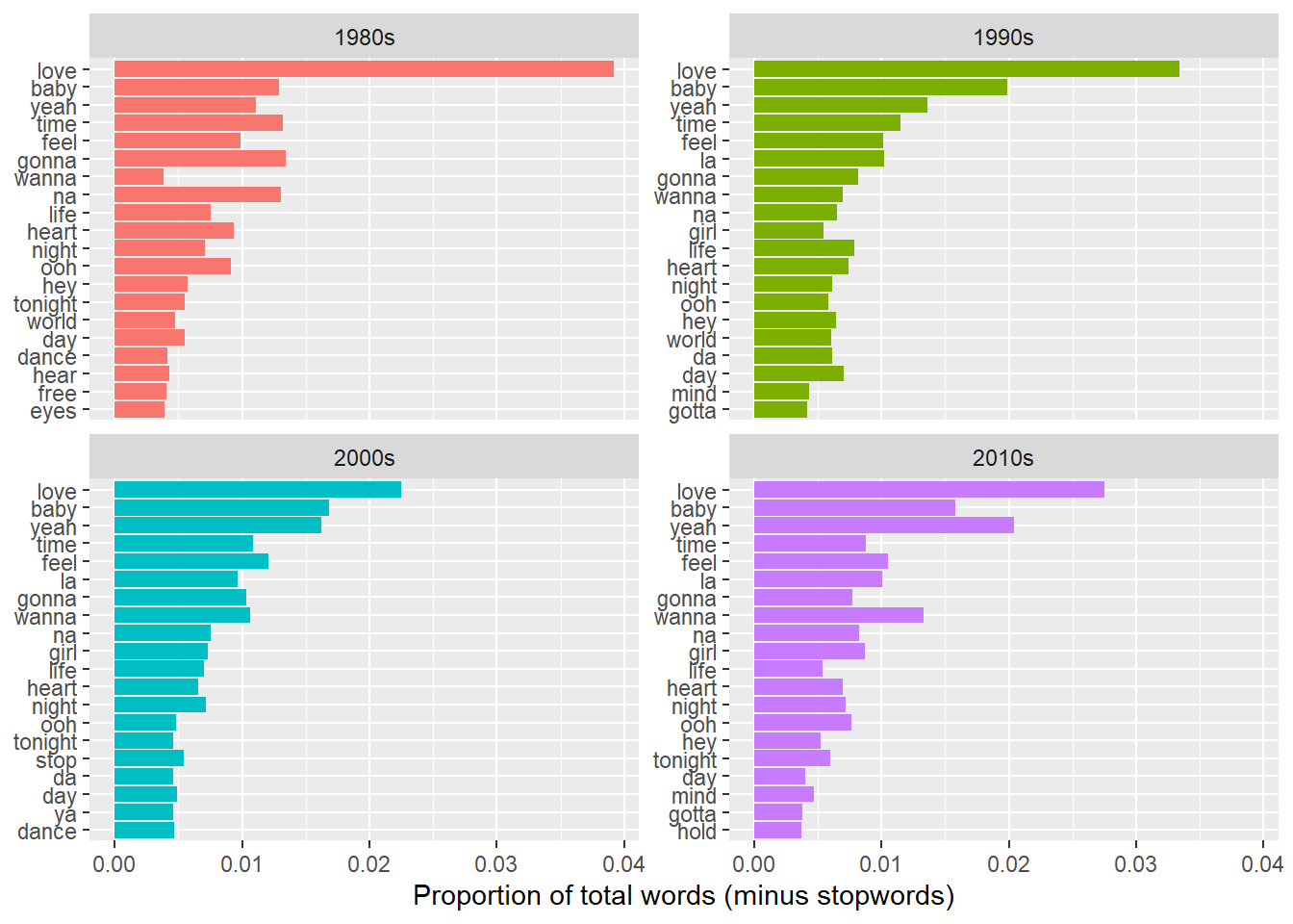

Yay, it’s love! Every decade! Although it’s more dominant in the 80s than the 2000s. Baby and yeah are perennial features, and for those times you’ve just run out of things to sing about, na (na na) is an enduring favourite, with la (la la) appearing from the 90s. There are a lot of similarities across the decades, with not many new themes appearing in the world of pop lyrics, and indeed few surprises – you could practically have guessed these.

Let’s do a more fine grained picture of how some of these have changed over time.

lyricsdata %>% 
  group_by(date) %>% 
  unnest_tokens(word, lyrics) %>% 
  anti_join(stop_words) %>%
  count(word) %>% 
  mutate(prop = n / sum(n)) %>% 
  filter(word == "love"| word == "baby" | word == "yeah") %>% 
  ggplot(aes(x = date, y = prop, colour = word)) + 
  geom_point(size = 1, alpha = 0.5) +
  geom_smooth(se = FALSE) + 
  facet_grid(word ~ .) + 
  ylab("Proportion of total words") +
  guides(colour = FALSE)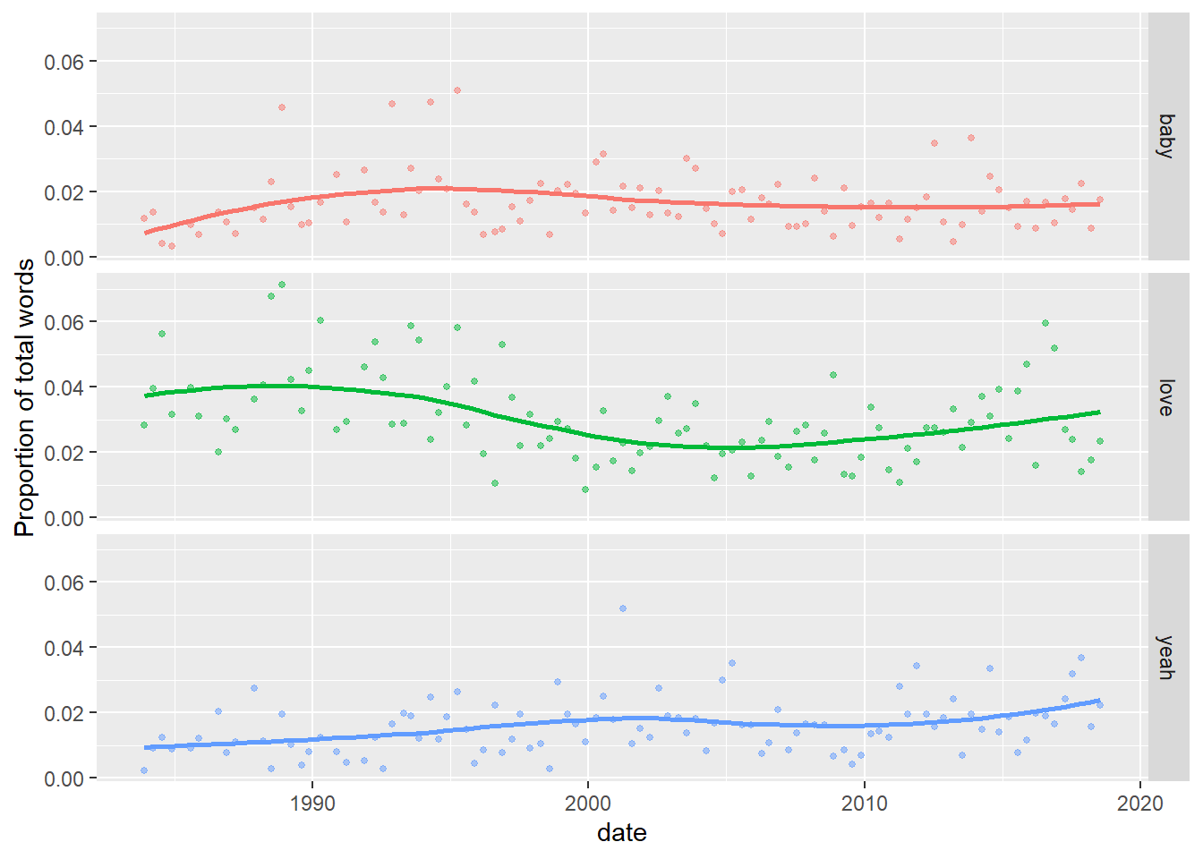

Each dot represents a Now! album, with a smoothed line drawn through them. It seems that love fell off in popularity for a while, but is now back on the way up. Yeah has also seen a small but steady increase, although baby may have peaked in the mid-90s. There’s not much that’s striking here in the way of trends though. If we want to know what distinguishes the songs over time, a comparison cloud is the way forward, which shows the words that are more prevalent in each decade compared with the others.

library(wordcloud)
library(reshape2)
lyricsdata %>% 
  filter(artist != "Eiffel 65") %>% 
  unnest_tokens(word, lyrics) %>% 
  mutate(word = str_extract(word, "[a-z']+")) %>%
  filter(!is.na(word)) %>% 
  anti_join(stop_words) %>%
  group_by(decade) %>%
  count(word) %>% 
  mutate(prop = n / sum(n)) %>% 
  acast(word ~ decade, value.var = "prop", fill = 0) %>% 
  comparison.cloud(max.words = 100, scale = c(3,0.5))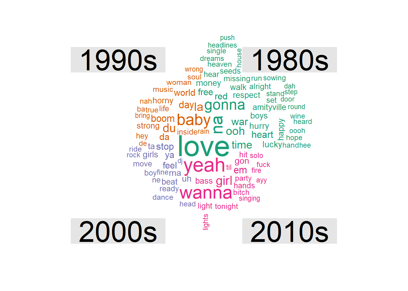

Some distinguishing features of each decade seem to be:

• The 1980s: political words - war, free, money (well it was the Thatcher era)
• The 1990s: nonsense words - de, ba, da ²
• The 2000: move-y, dance-y words - dance, move, rock
• The 2010s: ayy, obscenity!

Another thing you can do is look at the emotional tenor of each album or decade. One way to do this is using the AFINN sentiment lexicon, which assigns a sentiment score to about 2,500 common sentiment words; a positive score of up to 5, or a negative score down to -5. If we calculate the average score of all the sentiment words in each album, we get something that looks like this:

# need to download manually
afinn <- readRDS("afinn.rds")

lyricsdata %>% 
  unnest_tokens(word, lyrics) %>% 
  mutate(word = str_extract(word, "[a-z']+")) %>% 
  inner_join(afinn) %>%
  group_by(date) %>% 
  summarise(meansent = mean(value)) %>% 
  ggplot(aes(x = date, y = meansent)) +
  geom_point(alpha = 0.5) +
  geom_smooth(se = FALSE) +
  labs(colour = "") +
  ylab("Mean sentiment score")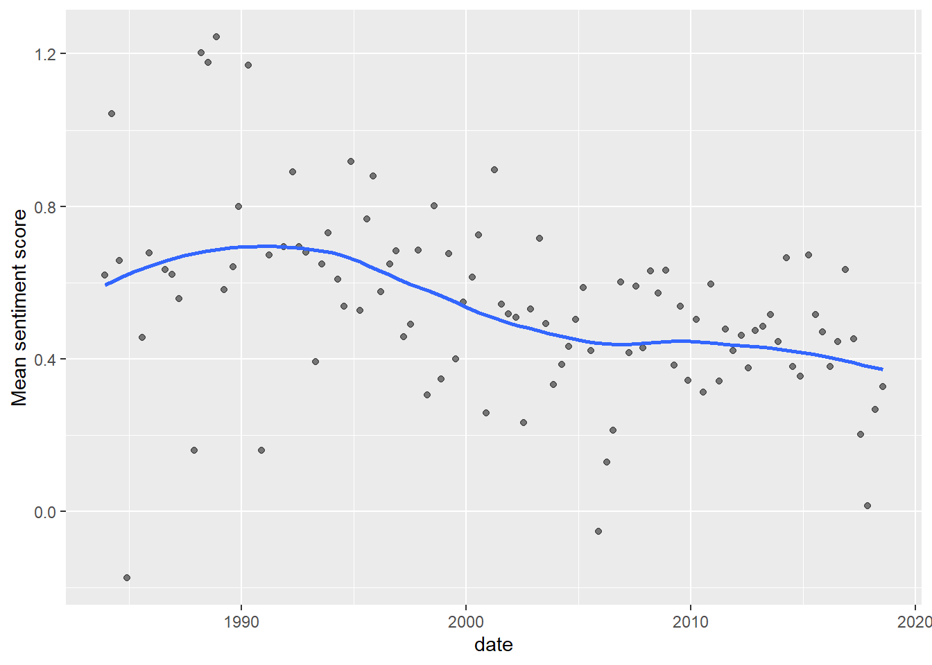

The average sentiment score peaked in the early 1990s and has been falling since then. Mean sentiment remains on the whole positive, but who knows what will happen if this trend continues?! 😱

You can also use the NRC sentiment lexicon to explore the presence of a range of emotions. What proportion of sentiment words in each decade’s lyrics fall into each category?

nrc <- readRDS("nrc.rds")

lyricsdata %>% 
  unnest_tokens(word, lyrics) %>% 
  inner_join(nrc) %>% 
  group_by(decade) %>% 
  count(sentiment) %>% 
  mutate(prop = n / sum(n)) %>% 
  mutate(sentiment = as.factor(sentiment)) %>% 
  ggplot(aes(x = fct_reorder(sentiment, prop), y = prop, fill = decade)) +
  geom_col() +
  xlab(NULL) +
  ylab("Proportion of sentiment words in category") +
  coord_flip() +
  facet_wrap(~ decade, scales = "free_y") +
  guides(fill = FALSE)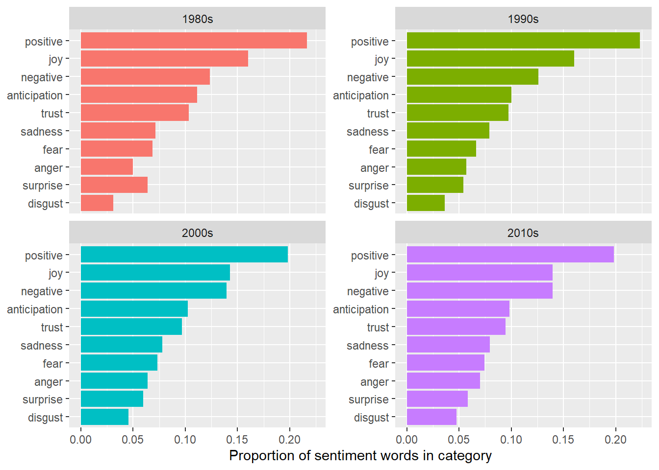

There is not much difference between the decades. The 80s were more surprised than angry, but the different emotions appear in very similar proportions across the decades, although you can see a drop off in positive words and increase in negative. Indeed, a look over time shows a divergence in the use of positive and negative words, followed by a narrowing.

lyricsdata %>% 
  unnest_tokens(word, lyrics) %>% 
  inner_join(get_sentiments("nrc")) %>% 
  group_by(date) %>% 
  count(sentiment) %>% 
  mutate(prop = n / sum(n)) %>% 
  filter(sentiment == "positive" | sentiment == "negative") %>% 
  ggplot(aes(x = date, y = prop, colour = sentiment)) +
  geom_line(alpha = 0.5) +
  geom_smooth(se = FALSE) +
  ylab("Proportion of sentiment words")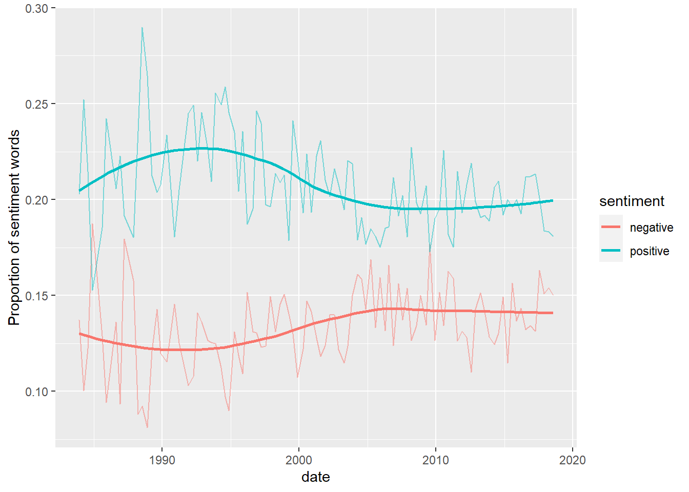

It might be interesting to bring in other information about the songs, like their chart position. Although everything on a Now! album is a ‘hit’, not everything will have reached the top of the charts, and there’s often some filler, which ideally you might want to filter out of the analysis. Equally, presence on a Now! album is not the only indicator of a song’s popularity – an alternative corpus could take top 10 songs over the same period. The guy who picks the songs for the Now! albums in the US says he uses a mixture of metrics and gut instinct, but I wonder if there are features that distinguish the songs that make it on.